Alpha Go Zero in depth

Introduction

A long-standing objective of artificial intelligence is an algorithm that learns superhuman competence by itself. If man succeeds in constructing such a system, then the repercussions of this discovery will be numerous and diverse and will change our daily life as human beings. However, it is not clear how we could give machines the ability to reason and understand the world around them. As of today, many systems, such as Amazon Alexa, or Google Home act as substitutes, allowing us to blossom with the limits of artificial intelligence, the fruit of an ungrateful training on a huge quantity of collected data. These advanced systems extract complex patterns hidden in the data in order to reproduce the human behavior. This is the case in the generation of speech, the understanding of images, or even the understanding of human desires. We are still a long way from an intelligent machine that understands us, and that would be the equivalent of a human being.

Earlier this month, DeepMind proposed a new algorithm capable of playing the game of Go without any assistance or human supervision. Despite the remarkable performance, it should be noted that this algorithm is based on the fact that the Go game is very well defined, providing a standard score for each move. For a machine, this corresponds to an environment that can be simulated quickly on a computer. Unfortunately, this is not the case for many complex human problems that are not yet well defined, nor modelable, and that above all require a certain knowledge and intelligence to be solved.

In the first section, we will review the origin of Reinforcement Learning (RL), as well as some of the algorithms used in Alpha Go In the second section, we will cover the two versions of Alpha Go, and their differences. Finally, in the last part, we will see potential applications to this new algorithm

On the origin of reinforcement learning

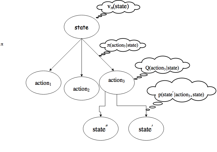
Reinforcement learning is a field of research where we teach agents to interact with an environment . This interaction required the agent to choose actions \(A\), that move the agent between states \(S\). Associated with each state is a notion of reward \(r\) that accumulate over the previous actions. The goal of the agent is to maximize the reward in the long term, instead of the immediate reward. When human creates the environment, they need to define how reward will be distributed. The agent needs to learn a policy \(\pi(action|state)\) that provide the next action to choose from a given state. When defining the rewards, there is a clear distinction to make with other machine learning technique: Rewards should not be given as a way to teach the human how to reach the ultimate goal, but instead, uniquely if the agent arrives at the goal. The agent will have to learn on its own what is the best way to succeed. For example, if you teach a robot to move from place \(A\) to place \(B\), you should never assign a reward to a certain path chosen.

Given what we have said in the previous paragraph, we want the agent to maximize the expected gain, i.e \(G_t = R_{t+1} + R_{t+2} + … + R_{t+T}\). But in case there is no terminal state, what we want instead is to maximize the discounted reward \(\sum_{k=0} ^ {\inf} \lambda^k R_{t+k+1}\). If we unified the last two equation, we find that \(G_t = \sum_{k=0} ^ {T-t-1} \lambda^k R_{t+k+1}\).

Reinforcement learning relies on the Markov assumption. As the policy \(\pi\) is defined as a probability distribution, we can apply the Markov property on it:

• The probability of moving to a new state \(s^{‘}\) is only conditioned on the previous state and the action taken.
• The expected reward after moving from \(s\) to \(s^{‘}\) with action \(a\) is only determined by the last three “objects”.

Although this may seem restrictive at first glance, the trick lies in modeling the problem, so that it will always respect the Markov property. For example, if stated in the problem, the last two states always condition the next one, then you have to go back to the modelisation, and make sure that these last two states are represented as a single one.

When the agent interacts with the environment, knowing and learning if it is good to be in this state, or if it is good to choose this action, is essential. For example, if we go back to our robot looking for a reference point, if to go to this point the robot can meet a river, it would be good that he learns to mark this place as “to avoid”. It leads us to see two functions:

• The value function: \(V_{\pi}(state) = \mathbb{E}(G_t|S_t=state)\) which gives us the expected reward to be in state \(state\)
• The state function: \(Q_{\pi}(state, action) = \mathbb{E}(G_t|S_t=state, A_t=action)\) which gives us the expected reward to be take the action \(action\) at state \(state\).

If the agent maintains an average for each state, or for each tuple (action, state), we know that if \(t\) goes to infinity, we would learn the true values. Sadly, expectation is for the theory, and in practise we work with approximate expectation using a sample of experimentations: $v_{\pi}(state) = \sum_{action} \pi(action|state) \sum_{state^{'}} p(state^{'}|action, state)[r(state^{'}, state, action) + \lambda v_{\pi}(state^{'})]$.

This formula, also known as the Bellman equation, is the foundation stone of all reinforcement learning problems. Here is a schema of what’s happening in the agent’s environment:

As previously mentioned, if the number of experiences goes on forever, we would learn the true values. That means we could order the policies: $\pi ^{'}\text{ is better than } \pi \Leftrightarrow v_{\pi^{'}}(s) >= v_{\pi}(s) \forall s$

In simple cases, if the Markov decision process is finished which means that the number of states and actions is finite, then the Bellman equations can be solved using a system of \(N\) equations, with N unknowns ((\(v_{\pi}(state)\text{ }\forall state\)). This property also assumes that the dynamics of the environment are completely known, i. e. \(p, r\) are constants. As a result, we can easily develop a policy that would maximize the value return on the discount reward (maximize long-term and short-term compensation). If we try to learn the state function \(Q\), it’s even easier because arg-max is hidden.

Dynamic programming

To solve the equations, we will use fast algorithms, or intermediate result storage techniques, such as dynamic programming used by some reinforcement learning algorithms. Some reminders and properties:

• The existence and uniqueness of the value function are guaranteed if \(\lambda\) is less than 1.
• If the system dynamics are known, the problem can be solved as a system with as many equations and unknowns as states

In our case, iterative methods are faster. Here is the new formula of the calculated value function iteratively: $v_{\pi}^{k+1}(state) = \sum_{action} \pi(action|state) \sum_{state^{'}} p(state^{'}|action, state)[r(state'{'}, state, action) + \lambda v_{\pi}^{k}(state^{'})]$. It is proved that as k goes to infinity, we learn the true values of \(v\).

Note that between two iterations, we can update efficiently the value function for all states using matrix multiplication operations, and cache the previous table, and the new one. As long as a value of a state is updated “significantly” (a hyperparameter must be defined), the algorithm continues.

The Policy Improvement Theorem tells us that \(Q(a, \pi^{‘}) >= v_{pi}(s) \forall s, \pi^{‘} > \pi, v_{\pi^{‘}}(s) >= v_{\pi}(s)\) This equation is very important has it links the value and state function, and is implicitly used in the results below.

We will now review two iterative algorithms used in practice to learn value functions, and get the optimal policy:

• Policy Iteration
• Value Iteration

The only difference between the two is that the Policy Iteration evaluates a new policy by updating the value function as a function of the current policy. In other words, the current policy function is used to determine the probability of moving from one state to another (see formulas in the link). The algorithm then updates the policy and then re-starts the evaluation until the policy no longer changes in the second phase. On the other hand, Value Iteration algorithm updates the value following a greedy policy that always chooses the most promising action. The returned policy is only updated at the end.
Seen in this way, Value Iteration requires less computation than Policy Iteration.

Monte Carlo methods

Until then, we have lived in a wonderful world, where the dynamics of the system were known, such as the final reward but also the transition table. Unfortunately, this is often not the case, and we need to rely on other methods to teach the agent a policy. Since Go has an unambiguous objective system and is a fully observable game, we can still use the first methods.

Perhaps in another blog, I would cover these methods, where bootstrap episodes of the agent in its environment are used to learn a policy. Looking for Time Difference Learning that merges Monte Carlo updates and dynamic programming, or Sarsa is a good rabbit hole journey start.

Recent progress in Reinforcement Learning with Neural Network as approximation functions

All games of perfect information have an optimal value function that can be determined using the reward at the end of the game. To solve this games, people have used search trees to compute recursively the optimal value function. For a game like Go, the possible sequence of moves possible grows exponentially as a function of the number of moves left. For Go, there are approximately 250 possible moves at every timestep, and 150 moves before the game finished. So the number of possibilities to evaluate is \(250^{150}\). To reduce the computation bottleneck, the depth and the width of the tree can be diminished using heuristics. For example, depth can be reduced by replacing some subtrees with an approximated value representing the expected reward under this subtree. For the width, sampling only actions from a golden policy allows only searching promising subtree.

Monte Carlo Tree Search¹ is a method to estimate the value of any state in a search tree using Monte Carlo rollouts. Monte Carlo rollout is a technique to traverse top to bottom a tree following a quick policy. One might try to pre-compute all the value function’s values, but this is no small matter, as it would require way more than all storage capacity in the world.

This is where neural networks comes in handy. Their importance lies in their ability to represent complex data, such as images, in an abstract way and to use them for predictive purposes, such as the estimation of a probability distribution over a set of actions. Here is an example ² of a neural network architecture that learns to play the Atari game from the screen printing of the game. The neural network produces a policy on possible actions, i. e. left, right, up, down, etc.

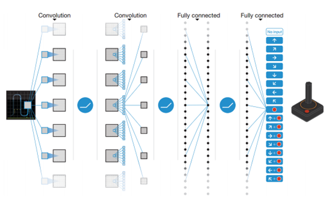
It should be noted that recent applications of neural networks as a function approximator have generated unprecedented performance in many areas. And DeepMind has been a major contributor to this discovery.

And in the industry, which uses learning reinforcement?

In a recent presentation, Andrew Ng, ranked the value of current methods of machine learning, pointing out that most of the value created comes from available supervised methods, followed by unsupervised techniques, and reinforcement learning techniques.

Reinforcement learning is not meant to play the last of classes until the end of the world, and recent breakthroughs in video games, open the way to potential applications in medicine, language understanding, and self-driving cars.

Alpha Go, deep neural networks and tree-searching

In their first attempt to break the game of Go ³, Deepmind developed a brand new training pipeline allowing a machine to play Go, with an honorary title of 9 dan. The training pipeline is decoupled in different stages, where new modules are added to the machine, allowing it to develop its game.

Supervised Training of the Policy Network

In the first part of the training, a neural network is trained to maximize the likelihood of picking the human move a, given any state. This training is completely supervised, using millions of positions from an open source dataset of master games, and the model is trained via gradient descent. This training produces two models: the \(SL\), used a the main policy network and a smaller one, less accurate but quicker, called \(FR\).

Reinforcement Learning of the Policy Network

Only when the supervised model has a low Mean Squared Error on the prediction of human movement, will it moves on to the next training step.

At this stage, the model is trained against a different version of itself. Opponents are randomly sampled from a pool of variants of SL. Over time, only the best models continue to play amongst themselves. All these models train and learn from their victories, i.e. defeats. The technique used is a variant of Policy Gradient methods. A reward function provides different signals to the model if the state is terminal, winning or losing. This signal is used in the gradient descent algorithm to optimize the parametrized policy network. If you want to know more, I suggest you take a look at this blog⁴

This new policy, called \(RL\), wins 80% against \(SL\).

Learning to evaluate the value network

The final step is the evaluation of board positions. In short, a model is trained to provide a score to each possible state in the game of Go. To do this, a neural network similar to \(SL\) learns to predict a single scalar value, instead of a policy, which is the state value. Training is supervised, as the sampled set consists of millions of distinct positions of parties played by different \(RLs\) against themselves. The value that the network must predict correctly is the final reward at any state in the game.

Improving performance by combining policy and value into an MCTS

At this stage of training, Alpha Go is composed of:

• A module that provides a policy over next actions,
• A similar module, quicker and simpler.
• A module that can evaluate the quality of a board position for a given player

At prediction time, a Monte Carlo Search Tree is built to evaluate the best move starting from the current state as a root. The tree has nodes as game state and edges as (state, action) tuple forming links between the game states. The child node is always the state at the next step. This architecture looks like the tree in Figure 1. An edge keeps tracks of multiple values: the joint probability \(p(state, action)\), the number of times the search traverses the edge, and the total and average action value.

Like all MCTSs, the tree is traversed in 4 successively repeated steps:

• The tree selects the edges to pass through using a randomly initialized Q action value first
• If a new node is discovered, the next action is selected using the policy predicted by \(SL\) for that state.
• Each node is evaluated by the value network, and also by a Monte Carlo rollout with \(FR\) as a quick policy.
• Finally, the Q action values are updated from bottom to top.

This is what hid behind the algorithm that defeated Lee Sedol last year in a competition followed by all Go fans, and geeks from around the world. Even though the performance stunned the whole world, it took no more than a year to see the new version, Alpha Go zero, capable of beating the previous version, Alpha Go Lee, 100 games to 0.

Alpha Go Zero⁵, you don’t change a winning team, you combine it!

The previous model, although very clever, demanded:

• Human Knowledge
• Several neural networks, two for policy function and one for position evaluation
• Requires dozens of GPUs to play

The new model simply requires:

• Trained from scratch without human expertise
• A single neural network
• Just 4 TPUs

The genius of Alpha Go Zero lies in the algorithm. This requires only one neural network, trained to provide a policy and a state value simultaneously.

For each new gameplay, the neural network is training to predict a probability for each possible movement and also the expected return value, win or loose. To correct its errors, the network is given additional time for reasoning, where it can take advantage of an MCTS to determine a better state value and strategy. The network corrects its predictions based on the values found during MCTS.

The procedure in MCTS is almost identical as the one in Alpha Go 2016:

• Build the tree from the current state of the game
• Go down until meeting a leaf node. On the way down, the edges are chosen using the Q value affected to the edges. A leaf node is either a terminal node or a node with a \(depth ~= 1500\)
• Compute the value function in this leaf state using the current neural network. If the game is finished, provide a synthetic evaluation of +1, -1.
• Backtrack this information up until the root and update the \(Q value\). Given that we chose an action \(action\), the \(Q value\) becomes the value function of the child state traversed divided by the number of times this state->action has been travelled.
• Repeat.

To save computation, MCTS is not re-initialized every time because the next move will use one of its subtree where the root node will be the current state.

The multi-objective loss has two terms:

• The squared error between the expected reward and the MCTS reward
• The cross-entropy between the neural network predicted policy and the MCTS policy
• (and an L2 regularization)

The dual objective regularizes the network to a common representation that supports multiple edge case.

When Alpha Go learns to play, the next move is sampled using a softmax over the MCTS predicted probabilities, controlled by a temperature term that balanced the trade-off between evaluation and exploration.

Finally, as training goes on, neural network weights are saved, and performance is compared between the most recent model and the previous models. Out of 100 games, the one that wins by a certain margin most of the games becomes the best player for the next iteration of self-training. During this generation phase, the player moves from a position to another, following an almost greedy policy driven by an MCTS search, where the action taken is the one that got visited mostly during the tree search.

Why does it work so well?

The structure of the networks used in AlphaGo Zero and Master have some great intuition that should hopefuly give some indication as to why a seemingly simpler system is capable of beating its more complex predecessor (AlphaGo Lee) however one would be forgiven for the confusion as to why AlphaGo Zero is able to beat Master so convincingly. The underlying principle that likely gives the systems increased capabilities is the sharing of features between the policy and value networks that allows the learning of much nicer features. However there is something else going on to explain why AlphaGo Zero is able to beat AlphaGo Master (which also shares this same idea) 100 games to 0. The difference between Master and Zero is that Master shares the training pipeline with AlphaGo Lee in that it is first trained on human games, it also uses some hand crafted features from the earlier versions. AlphaGo Zero has none of this and is trained entirely using reenforcement learning. At first glance, one might assume that this would be less effective due to a less informative training signal but that is not the case, but why? This next section is purely speculation, but I expect it actually has to do with a kind of local minima that has been found by human gameplay such that no small permutations to the human learned technique is able to greatly increase its capabilities.

So why should we care anyway?

“the rules of Go are so elegant, organic and rigorously logical that if intelligent life forms exist elsewhere in the Universe, they almost certainly play Go”.- Edward Lasker

Before alphago beat Lee Sedoul it was to be believed that a computer beating a world champion was at least a decade away, a game in which humans dedicate their lives to mastering was conquered by a program written by people who themselves would not stand a chance. Is this a defeat for go or a giant leap for reinforcement learning and by extension AI? AlphaGo zero has been able to achieve in a matter of days the knowledge that took Go masters and scholars thousands of years of collective intelligence to develop. It was also shown that many of the techniques that alphago developed for its self are identical to strategies that have been developed by go players over this time period. Alongside these however, alphago was able to develop its own strategies that have not before been seen by the world of go, this acomplishment alone is a truly tremendous result and one that DeepMind will forever have their flag marked upon. (like IBM do with chess)

The nice biproduct of applying machine learning to games is that it is capable of hitting the wider media and allowing regular people to get a real world grasp of the state of research in AI and allow people to get excited about a field that so often receives only scare-mongering or overstated claims by the media.

AlphaGo Zero offers a truly beautiful solution to the problems solved with the original alphago, the idea of shared representations is both logical and efficient. I would even go so far to say that it makes the already beautiful original alphago look clunky.

I think one of the real contribution of this research is the demonstration that reinforcement learning upon earlier versions of its self is on its own capable of truly astonishing results, in fact much better than was achieved by learning from master games. This coupled with the novel approach of merging policy and value networks has resulted in the fantastic results that we see here. The hope is that this will guide us into a realm where reinforcement learning is not only feasable to be used as a final “fine tuning” as it so often is but a method that can be deployed from scratch to extremely complex problems, given only a simulator of the system we wish to master.

My concern with this however is that the game of go offers us a faithful, accurate and importantly easy-to-compute simulator of the discrete and fully observable world of go. This scenario is one that we are not often forunate enough to have in the most valuable real world applications of reinforcement learning.

This said, there are some exciting applications that can be easily simulated such as control systems for autonomous vehicles or robots both of which are simulatable with a reasonable reliability. But these systems still leave the unanswered question for alphago as to whether it can generalise over the non-observability and stochasticity of these systems. One thing is for sure though, this work from Deepmind will be built on and utilised in all kinds of novel and exciting ways over the coming months and years and hopefully bring us closer to solving some of the most important problems faced by the world.

Acknowledgments

A big thank you to Ben Townsend for his precious proofreading and sharing his point of view on the repercussions and applications of Alpha Go Zero.

Bibliography