Image Generation with BEGAN and Skip-Though vector.

Skip Thought Vector

Skip thought vector is a powerful technique to map semantically and similar syntactic sentences to same vector representation. Since 2015, the paper has already been cited more than 250 times, which is entirely deserved.
Until 2015, the traditional deep learning ways to compute sentence embedding was to learn composition operators that maps (word2vec) word embeddings to sentence representations using diverse architecture such as recurrent network ¹, recursive network ², and also convolution neural network ³. All these models fall under the supervision tasks; they required a loss function at the bottom of the neural network to be trained. Hence they are biased towards their respective functions.
Skip though vector is completely unsupervised, and is often compared to word2vec but at a sentence level.

In essence, what skip thought vector is like the continuous skip-gram architecture of word2vec, but here a sentence is used to predict its surrounding sentences. Training data is in form of current sentence $s_i$, the next sentence $s_{i+1}$ and the previous sentence $s_{i-1}$. The current sentence is encoded at the word level, using a shared word2vec dictionnary between all encoder/decoders, and a classical GRU cell:

At the end, the last output vector $h_i$ is retrieved and will be used for predicting the surronding sentences. For this tasks, two decoders are shared which do not shared weights. Instead of a vanilla GRU cell they introduced three matrices $C_r$, $C_h$, $C_z$ to bias the update, reset gates and the hidden states. Here are the formula. During decoding, at timestep $t$, we have:

$r^t = \sigma(W_r^{dec} x^{t-1} + U_r^{dec} h^{t-1} + $ $C_r$ $h_i)$
$z^t = \sigma(W_z^{dec} x^{t-1} + U_z^{dec} h^{t-1} + $ $C_z$ $h_i)$
$h^t = tanh(W_h^{dec} x^{t-1} + U_h^{dec} h^{t-1} + $ $C_h$ $h_i)$

As usual seq2seq models, the probability of having the word $w_t^{i+1} = w_k$ in the next sentence at timestep $t$ is computed using a softmax (or a sampling softmax), and a learnable dictionnary matrix for each words.

That’s the theory, now how does it perform on MS Coco caption dataset. Here is some representation in 3D of the vector obtained for every caption. I used t-sne for the dimensionality reduction.

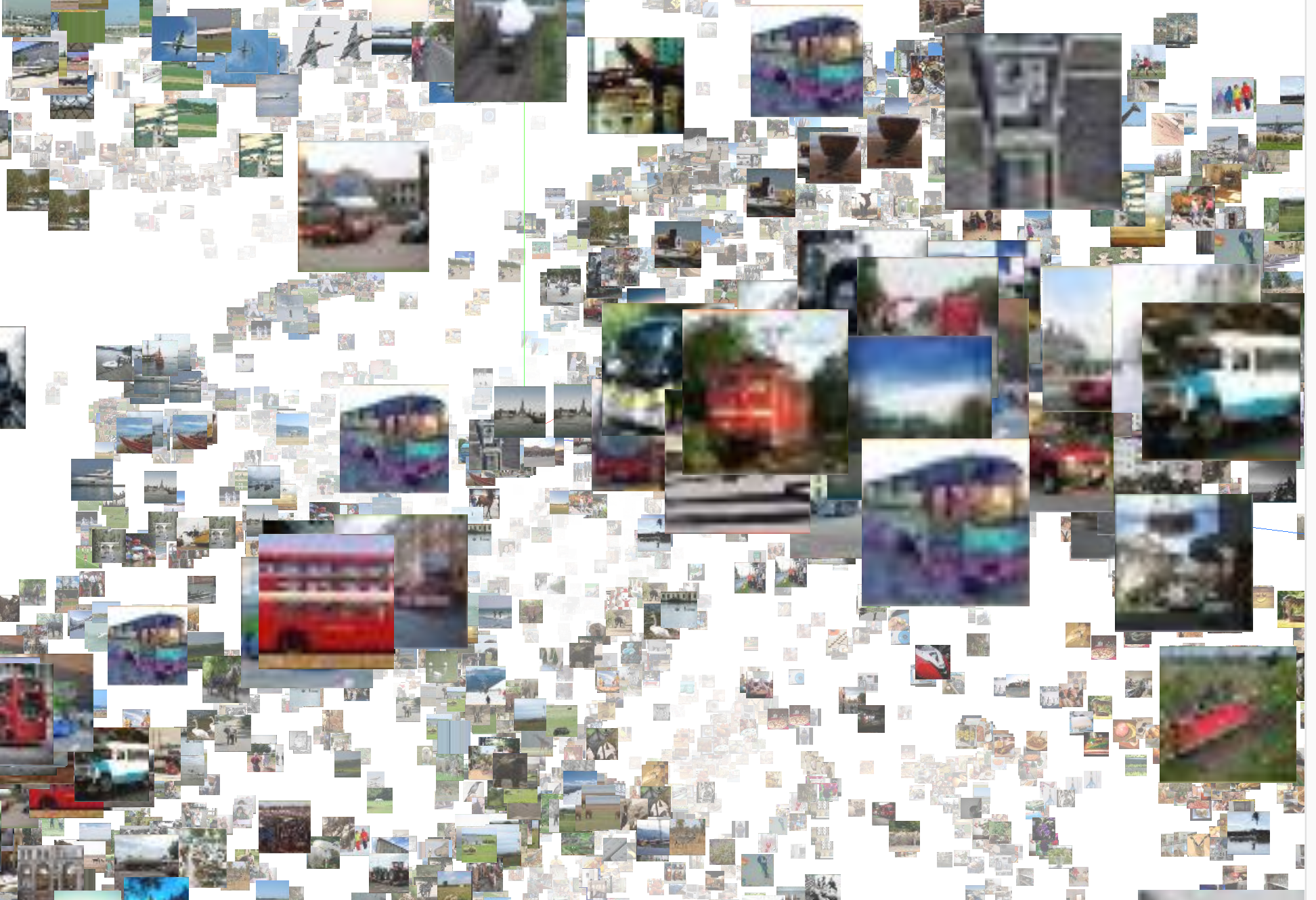
Figures 1: Closest caption to "A cat laying on top of a computer keyboard"

Figure 2: Visualisation of the manifold of bus

I have a lot of other examples, but this proves that skip-thoughts vector has captured some syntactic and semantics about captions. We’ll use them to try to generate images with the next architecture: a BEGAN.

Boundary Equilibrium Generative Adversarial Networks

Introduction to Generative Adversarial Models

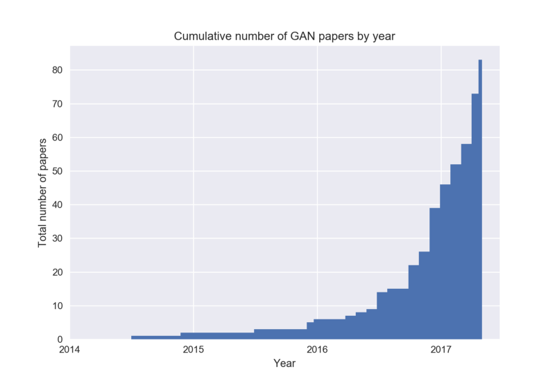
GAN, GAN, GAN, there has been a huge craze for them because they were able to produce some of the nicest looking samples. This graphic resumes all about the success of the Generative Adversarial Model.

Generative Adversarial Model ⁴ are model that are able to learn a data distribution and allows to sample from it. The vanilla GAN objectives can be thought of as a minimax game played between the Generator ($G$) and the Discriminator ($D$) with the dueling objectives : $\min_{G}\max_{D} V(D,G)$, where:

$V(D,G) = E_{x \sim p_{data}(x)}[\log D(x)] + E_{z \sim p_{z}(z)}[\log(1-D(G(z)))]$

Current issue with GANS

Unstable training

GANs training is giving a hard time to train because, defined as a zero-sum game, if one player becomes too powerful the “game is over,” and gradients could vanished before reaching the Generator.

Mode collapse

Another big issue of GANs is mode collapse. The intuition for this is to look at another formula derived from the minimax equation. Finding the optimal $p_G(z)$ among a class of generative models corresponds actually to minimizing the Jensen-Shannon: $JS(P\|\|Q) = \displaystyle{\frac{1}{2}KL(P \|\|M) + \frac{1}{2}KL(Q\|\|M) }$

where

$M$ is a mixture of $P$ and $Q$: $M = \frac{1}{2}(P + Q)$
and KL is the Kullback Leibler divergence, defined in a continous space as $\int_{-\infty}^{\infty} q(x) log(\frac{q(x)}{p(x)}) \, \mathrm{d}\mu_x$.

How does the KL and the reverse KL divergence behaves?

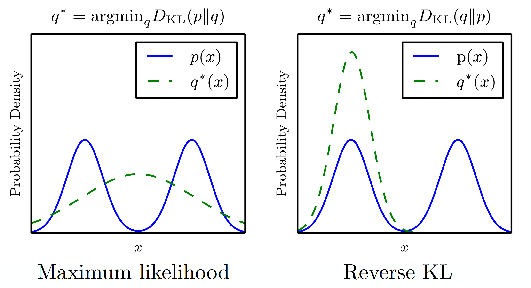
Figure 3: Approximated distribution given KL or reverse-KL training

In $KL(P|Q)$, if $P$ is multimodal, then the optimal $Q$ will try to cover all modes, putting mass at point $X$ of probability $P(X) = 0$. It is because, in the formula of the $KL$, $Q$ is not penalized for putting mass on thoses points. This means that the generative model trained on KL divergence will tend to overgeneralize.
In $KL(Q|P)$, the reverse KL divergence, $Q$ “leads” the training, so wherever $Q$ doesn’t put any mass, it is not penalized. As a result, the optimal $Q$ is often at the largest mode of $P$, ignoring other modes. We can see the dynamic of the training: as soon as the approximated distribution puts correct mass on a mode of $p$, it will then try to fit perfectly the curve at that point, avoiding introducing unplausible samples, at the cost of missing other plausible samples. Training might get stuck producing only blue estate car.

So we could think because GANs is a combination of both KL, training them will behave halfway between the two extreme behaviors. Regrettably, because the reverse KL is super hard to optimize, and not well defined wherever $P$ has a low dimensional support, this statement is false.

No measure of convergence

Finally, with vanilla GANs, there is no way to measure convergence of the training, because the training loss doesn’t mean anything. A recent paper, WGAN ⁵, tackles this issue by introducing a new loss function, which is showed to correlate well with the perceptual quality of the sample generated by $G$.

The new loss function introduced to use the Earth Moving distance defined as:

“Probability distributions are defined by how much mass they put on each point. Imagine we started with distribution $Pr$, and wanted to move mass around to change the distribution into $Pg$. Moving mass m by distance add costs $m \cdot d$ effort. The earth mover distance is the minimal effort we need to spend.” From Read-through: Wasserstein GAN

Another significant contribution of this paper is that it allows for training the Discriminator until optimality, and then used it to get “good” gradients for training the Generator. However, one drawback of this technique is that for the convergence property to hold, they had to enforce k-Lipschitzness for the function approximator (i.e., G and D). They decided to do it by clipping weights, which results in slow training and less capacity for the neural networks. In the next paragraph, we will see that BEGAN uses the different hypothesis to remove this constraint.

BEGAN

Introduction

In essence, BEGAN uses an auto-encoder as a discriminator. With the auto encoder, BEGAN optimization tries to match the distribution of the errors instead of the usual used samples distribution.

For training the auto encoder, they used a L1 loss (i.e $L(v) = |v - D(v)|^1$ where $v$ is the input of the AE and $D(v)$ the output).

Given the hypothesis that the loss at the pixel level is independent and identically distributed (i.e $\forall x_i\text{ a pixel, then }p(L(x_i), L(x_j)) = p(L(x_i)) p(L(x_j))\text{ }j \neq i, $, and all $L(x_*)$ are generated from the same distribution, then by using the Central Law Theorem, we can state, that as the number of pixels increased, the distribution can be approximated by a Gaussian distribution $\mathcal{N}(\mu, \sigma)$.

We can then find a closed form for the squarred Wassertein distance $W$ between two Gaussians, and under certains constraints have a nice form of it:

$W(m_1 \propto \mathcal{N_1}, m_2 \propto \mathcal{N_2})^2 \propto \|\|\mu_1−\mu_2\|\|_2^2$

I think they started their demonstration with the squared Wasserstein distance $W_2$ for Gaussian distribution formula because there exists an excellent established formula for it ⁶. See here. So the results holds for $W_2$, but not for $W_1$, which is nevertheless upper-bounded by $W_2$. Now, their method probably minimizes $W_1$ at the same time it would have minimized $W_2$, but the connection is not cleared to my mind.

So as we said earlier, we are going to assume our loss distribution is Normal and derived the math using this hypothesis. If we defined $m_1$ as the auto encoder loss of the true image $L(x)$ and $m_2$ the loss of the fake sample $L(G(z))$, $z$ being a random uniform latent vector.

We can write the loss function as a GAN objective with two losses:

$L_D = L(x) - L(G(z)) \text{ for } \theta_D \text{ (weights of the auto encoder)}$ $L_D = L(G(z)) \text{ for } \theta_G \text{ (weights of the generator)}$

If you read the WGAN paper, both losses are quite similar, except that in BEGAN, it does not require any Lipschitzness constraints, because we assumed we had a Gaussian distribution, which gives us a different form of the Wasserstein distance.

In Tensorflow this will be written as:

def autoencoder_loss(out, inp, eta=1):
    diff = tf.abs(out - inp)
    return tf.reduce_sum(tf.pow(diff, eta))

mu_real = autoencoder_loss(D_real_out, D_real_in)
mu_gen = autoencoder_loss(D_gen_out, D_gen_in)
D_loss = mu_real - k_t * mu_gen
G_loss = mu_gen

Did you notice the $k_t$ in the code? Well, this has also been introduced in the BEGAN paper, and it will help ensure the stability of training.

Control Theory and Convergence

In game theory, the Nash equilibrium is a solution concept of a non-cooperative game involving two or more players in which each player is assumed to know the equilibrium strategies of the other players, and no player has anything to gain by changing only his or her strategy. Similarly, in GANs, a possible equilibrium occurs when:

$\mathop{\mathbb{E}}(L(x)) = \mathop{\mathbb{E}}(L(G(z)))$

If this equilibrium occurs, then G would have won over D, producing no distinguishable sample from the real distribution, and we don’t want this. We always want to maintain the two players, G, and D, “in the game.” To doing so, we will try to maintain this ratio to a specific value (Let’s call it $\gamma = \frac{\mathop{\mathbb{E}}(L(G(z))}{\mathop{\mathbb{E}}(L(x))}$) during training.

Gamma will be an hyperparameter between $[0, 1]$, thus, and you’ll see soon, we wil enforce $\mathop{\mathbb{E}}(L(x)) > \mathop{\mathbb{E}}(L(G(z)))$)

If $\gamma$ is close to 1, then the expected losses are similar, hence D is trying to improve at its auto-encoding tasks on both distribution, resulting in a more diverse output.
If $\gamma$ is small, then $\mathop{\mathbb{E}}(L(x))$ becomes large, which means that the Discriminator is focusing more on improving its loss w.r.t to the true image. Diversity is impacted. Figure 4: Generated images given different gamma values

During training, we want to maintain the ratio of expectation to a fix value, which can be written as a equation constraint:

$\gamma = \frac{\mathop{\mathbb{E}}(L(G(z))}{\mathop{\mathbb{E}}(L(x))}$ $\gamma \mathop{\mathbb{E}}(L(x)) - \mathop{\mathbb{E}}(L(G(z)) = 0$

Proportionnal Control Theory can do the job for us to adapt this ratio during optimization dynamically. The algorithm will update a factor $k_t$, at each time step t, that will adapt depending on how far we are from the optimal desired ratio of expectation.

$L_D = L(x) - k_t L(G(z))$ $L_D = L(G(z))$ $k_{t+1} = k_t + \lambda_k (\gamma L(x) - L(G(z))) \text{ for each timestep }t$

If $k_t$ becomes too large (because $L(x)$ is larger than $L(G(z)))$, then the discriminator loss will be forced to focus more on $L(G(z))$, and vice-versa, so none of the players can win the game.

Training procedure also becomes simultaneous, while still being adversarial. There is no need to balance training period between them manually.

Finally deriving a convergence measures becomes possible. We know we want to minimize the reconstruction loss on the correct image, and also maintain the equilibrium constant, thus, if the sum of this values $L(x) + |\gamma L(x) - L(G(z))|$ gets low, then it is good proxy to say training converged.

Results

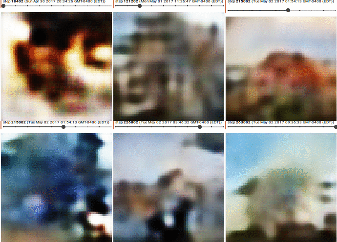
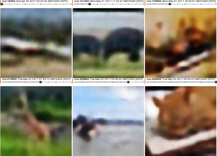
MSCOCO with Conditionnal BEGAN with gamma = 0.55, norm 1

Generated Images Evolution

Reconstruction of Generated Images Evolution

Reconstruction of True Images Evolution

True Images Evolution

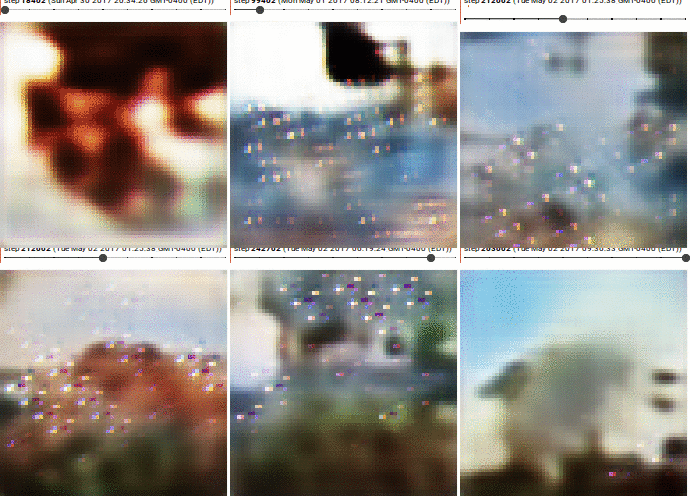
MSCOCO with Conditionnal BEGAN with gamma = 0.55, norm 2

Generated Images Evolution

Reconstruction of True Images Evolution

True Images Evolution

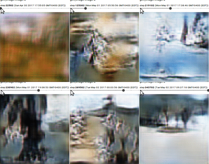
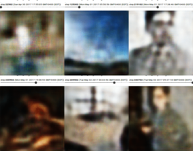
To be fair, I didn’t expect great results. Original papers were trained on human faces; I trained it on a complex multimodal distribution, where different samples might share no similarities. It makes the job hard for the generator to pick which “type of image” to generate, hence resulting in artifacts. If I have more time, I’ll train BEGAN on LSUN dataset :)

Code

All the code for reproducing the experimentations is here

Footnotes

1:: This is mostly because when minimizing a $L_2$ loss, this is the same as maximizing the log likelihood of a Gaussian distribution. However, images are usually complex distribution, with multiple modes. For example, there is not a single way to represent a car (it can be blue, yellow; it can be large, with or without a rooftop, and images are usually taken from a wide range of camera angle), thus doing ML can be interpreted as taking the average of all the representation of car to generate a new one in the manifold of automobiles, resulting in blurry images. 2:

Bibliography

Long short-term memory from Sepp Hochreiter and Jürgen Schmidhuber. ↩
Recursive deep models for semantic compositionality over a sentiment treebank from Richard Socher, Alex Perelygin, Jean Y Wu, Jason Chuang, Christopher D Manning, Andrew Y Ng, and Christopher Potts ↩
A convolutional neural network for modeling sentences from Nal Kalchbrenner, Edward Grefenstette, and Phil Blunsom. ↩
Generative Adversarial Networks from _ Ian J. Goodfellow, Jean Pouget-Abadie, Mehdi Mirza, Bing Xu, David Warde-Farley, Sherjil Ozair, Aaron Courville, Yoshua Bengio_ ↩
Wasserstein GAN from Martin Arjovsky, Soumith Chintala, Léon Bottou ↩
The Fréchet distance between multivariate normal distributions from D.C Dowson, B.V Landau ↩