The Hyperband Algorithm.

In this article, we will review a recent approach to hyper parameter search.

Why a new hyper parameter search algorithm?

In the past month, I’ve been spending some time on Bayesian optimization, and they’ve become my favorite way to go for hyper parameter search. I’ve done a simple module for using Spearming software (an implementation of Bayesian optimization) in the context of deep learning using Lasagne Library. In the context of hyper parameter optimization, I also tried a reinforcement approach following Designing Neural Network Architecture using Reinforcement Learning, without success (see code . One of my claims is that it required way too much computational resource that many machine learning researcher can’t afford. At the same point, even with good GPUs, it was time-consuming, because it required training neural network for some epoch ruled by early stopping, and I realized that most of the training configuration where not promising since the beginning. The only way to avoid this nonpromising expansion was to whether trained only promising neural network architecture, or hard-coded rules in early stopping method for nonpromising training.

Instead, in HYPERBAND, they explore a different direction for hyper parameter optimization that focuses on speeding up configuration evaluation. I decided it was the moment to try it. By adaptively allocating these resources, their approach aims to examine orders of magnitude more hyper parameter configurations than approaches that uniformly train all configurations to completion, thereby quickly identifying good hyperparameters.

First, they proved that Bayesian optimization (SMAC and TSE) consistently outperforms random sampling, but by a small gap. However, given more capacity, let’s say two computer instead of one, random search always produces better results.

This is their primary motivation for improving random search, by allocating different amount of resources for particular hyper parameter configuration.

SuccessiveHalving

HYPERBAND is an extension of the SuccessiveHalving algorithm. Here is a simple pseudo-python code of the last one.

budget = 1000 # time or nb_epochs to allocate for hyper parameter search 
              # Note that this we can do extend search without exploding the budget
              # by parallelizing tasks
nb_configuration = n = 30 # number of configuration to explore

all_configurations  = [get_new_configuration() for _ in range(nb_configuration)]

while len(all_configurations) != 1:
    # Save current proxy score for configuration selection 
    score_configuration = {}
    # Saved currently trained model
    saved_model = {}
    
    # Reduce budget
    budget =  budget / (len(all_configurations) * (log(nb_configuration) / log(2)))
    for configuration in all_configurations:
        # Create a new model the first time,
        # then restore the model
        if configuration in saved_model:
            model = saved_model[configuration]
        else:
            model = create_new_model[hyperparameter=configuration]
        
        model.train_algorithm(until_epoch=model.last_epoch + budget/len(all_configurations))
        
        saved_model[configuration] = model
        score_configuration = model.get_validation_score()

    # Sort model
    index_sorted = arg_sort(score_configuration)
    all_configurations = all_configurations[index_sorted]

    # Save half of the model for next round
    saved_model = saved_model[:len(all_configurations) / 2]

Notes

It is easy to show that the allocated budget for the algorithm does not exceed the budget:

where \(P_k =\) len(all_configurations), and \(k\) is the current iteration of the algorithm.

In practice, the optimal allocation strategy is unknown because we do not have knowledge of the envelope functions nor the distribution of terminal losses. Hence at the beginning, it may be unfair to differentiate model based uniquely on the first iteration validation curves. A simple example is to compare gradient descent based model with low learning rate: they usually perform badly at first before converge slowly to a better solution. SuccessiveHalving will usually throw them at the first step, without further consideration. Not desired.

Pseudo Code

There are two parameters to set for the algorithm

• \(R\): The maximum number of time/epoch to allocate to a single configuration. I think this is more relevant than having to set a global budget. In the context of Machine Learning problem we often set a fixed number of epochs and used upon some early stopping technique.
• \(\eta\): The proportion of configuration to discard at each iteration.

Now here is the algorithm:

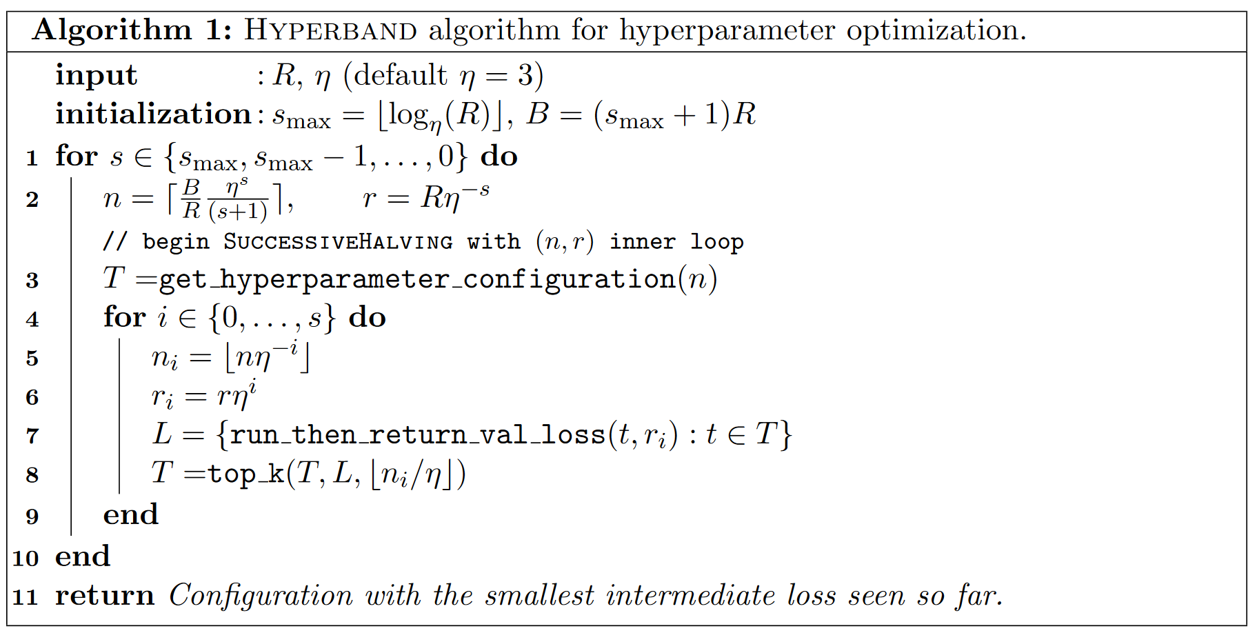
There are two loops in the algorithm.

• The first outer loop computed (\(n\) and \(r\)).
• The second inner loop computed a full iteration of a SuccessiveHalving.

At the beginning, \(n\) is set large for early value of \(s\), and it’s the opposite for \(r\). Hence in the inner loop, it will allow exploring a lot of configuration a few iteration very quickly. However as \(s\) decreased (outer loop), \(r\) is set larger, but n decreased. hence fewer model will be tried, but those will be tried longer. It will allow model that performed great lately to be revealed….

Bibliography