Seq2Seq Models for Short Answer Generation.

Seq2Seq Models for Short Answer Generation

Recurrent Neural Networks (RNN) are a particular kind of artificial neural networks that are specialized in extracting information from sequences. Unlike simple feedforward neural networks, a neuron’s activation is also dependent from its previous activations. It allows the model to capture correlations between the different inputs in the sequence.

However, this type of architecture can be very challenging to train, partly because it is much more prone to exploding and vanishing gradients ¹. These problems can be overcome by choosing more stable activation functions like ReLU or tanh and by using more sophisticated cells like LSTM and GRU, which involve more parameters and computations than the vanilla RNN cell but are designed to avoid vanishing gradients and capture long range dependencies ².

In the recent years, RNNs along with the mentioned strategies have been able to achieve state of the art level of performance on many challenging tasks like conversational models ³, machine translation ⁴ and automatic summarization ⁵. In this project, we implement a sequence to sequence (Seq2Seq) model using two independent RNNs, an encoder, and a decoder. We use the Cornell Movie dialog data set to train a short text answering model similar to the work of Shang et al. ⁶. We also explore the use of similar models on custom data sets of Facebook-Messenger conversation histories.

A bit of theory

Recurrent Neural Networks

In a regular RNN, at time-step \(t\), the cell state \(h_t\) is computed based on its own input and the cell state \(h_t\) that encapsulates some information from the precedent inputs :

$$h_t = f(W^{hx}x_t + W^{hh}h_{t-1})$$

In this case \(f\) is the activation function. The cell output for this time-step is then computed using a third series of parameters \(W^{hy}\) :

$$y_t = W^{hy}h_t$$

With LSTM or GRU cells, the core principle is the same, but these type of cells additionally use so-called gates that allow to forget information or expose only particular part of the cell state to the next step.

Sequence to Sequence

Sequence-to-sequence models (or RNN encoder-decoder) have first been introduced in 2014 almost simultaneously by two different research groups ⁷, ⁸. They have recently emerged as the new way-to-go for various generative tasks. The principle of Seq2Seq architecture is to encode information on an input sequence \(x_1\) to \(x_T\) and to use this condensed representation known as context vector to generate a new sequence \(y_1\) to \(y_{T^{‘}}\). Each output \(y_t\) is based on previous outputs and the context vector :

$$p(A|Q) = p(y_1, y_2, ..., y_{T^{'}}|x_1, x_2, ..., x_T) = \prod_{t=1}^{T^{'}}p(y_{t}|c_t, y_1, ..., y_{t-1})$$

The loss \(\ell\) is the negative log-probability of the answer sequence \(A = [y_1, …, y_{T^{‘}}]\) given the question sequence \(Q = [x_1, …, x_T]\), averaged over the number \(N\) of \((Q,A)\) pairs in a minibatch :

$$\ell = -\frac{1}{|N|}\sum_{(Q,A)\in N} p(A|Q)$$

Multiple layers of RNN cells can be stacked over each other to increase the model capacity like in a regular feedforward neural network.

The following figure presents a Seq2Seq model with a two layers encoder and a two layers decoder:

It is also common to have different weights for encoder and decoder cell:

$$W^{h*}_{encoder} \neq W^{h*}_{decoder}$$

Attention Mechanism

Theoretically, a large enough and well-trained model should be able to perform well on predicting the best decoding sequence given the encoding ones. Indeed, neural networks are universal function approximators ⁹ , which means they theoretically can model any function, even the conditional distribution \(p(y_1, y_2, …, y_T|x_1, x_2, …, x_T)\). However, in practice, we don’t have unlimited data, so we need to have a proper inductive bias, that will allow the network to learn to model accurately with a reasonable amount of data.

The first bottleneck with the previous model is that all the relevant information to decode is fed through a fixed size vector. When the encoding sequence is long, it often fails to capture the complex semantic relations between words entirely. On the other hand, if the fixed size vector is too large for the encoding sequence, this may cause overfitting problem forcing the encoder to learn some noise.

Furthermore, words occurring at the beginning of the encoding sentence may contain information for predicting the first decoding outputs. It is often complex for the model to capture long term dependencies, and there is no guarantee that it will learn to handle these correctly. This problem can be partially solved by using a Bi-Directional RNN (BD-RNN) as the encoder. A BD-RNN will encode its input twice by passing over the input in both directions:

It allows for hidden representations at each timestep to capture both future and past context information from the input sequence.

However, to better overcome the information bottleneck and long-term dependencies limitations, attentions model have been introduced. The basic idea of attention is that instead of attempting to learn a single vector representation for each sentence, we keep around vectors for every word in the input sentence, and reference these vectors at each decoding step.

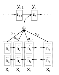
• Outputs from the encoder cell are usually used as attention vectors. We will call them \(h_{j}\text{, } \forall j \in [1, T]\). From the original paper ¹⁰ equation, a 1-layer MLP is used to learn a combination of the decoder previous hidden vector \(s_{t-1}\) and all the attention vector output \(h_{j=1,…,T}\).

  $$b_{tj} = v_{a}^{T}tanh(W_{a}s_{t-1} + U_{a}h_{j})$$

  The optimization algorithm should learn to produce large \(b_{tj}\) when the \(j\)th attention vector is relevant for decoding the \(t\)th token.

• The \(1D\) vector \(b_{t} = (b_{t0}, … ,b_{tT})^T\) is then passed through a softmax function. One reason to compute the softmax is to keep the math as correct as possible. Removing the softmax may cause values in $b_{t}$ to increase continuously with training while competing against each other to be the most relevant vector to use. Hence, we can see the softmax function as a regularizer. $\alpha_{tj} = softmax(b_{tj}) = \frac{exp(b_{tj})}{\sum_{k=1}^{T} exp(b_{tk})}$

• The final context vector is computed as a convex sum of every attention vector:

  $$c_t = \sum_{j=1}^{T}\alpha_{tj}h_{j}$$

  This vector is finally concatenated with the decoder input. The following figure summarizes how the attention mechanism works:

Seq2Seq tricks

Beam Search

Beam search is a well-known heuristic search algorithm, which has been widely adopted in large systems with an insufficient amount of memory to store the entire search tree. In the context of sequence generation, and when a model is already trained, the decoder predicts the next token as the

$$\arg\!\max_{k \in |K|}(softmax(y_{tk}))$$

where \(|K|\) is the decoder vocabulary size. Because the model has been trained with maximum likelihood, the most probable answer is not always the best, and maybe the second best choice of word will condition a better answer. Keeping the \(M-\)best word prediction at every time step is what beam search does.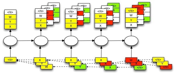

Sample softmax

During training, the predicting token \(y_k\) is computed with the softmax function, and as |K| is usually larger than the RNN cell hidden size |h|, a dictionnary matrix \(W \in \mathbb{R}^{|K|, |h|}\) is constructed. Every row \(w_k\) becomes the learned representation of a token \(y_k\).

In essence, the softmax forces the learning algorithm to orientate row vector \(k\) of \(W\) in the same direction of the output of the cell when \(k\) should be the predicted token, so that the future softmax function will return a larger value at index \(k\).

However, as \(|K|\) becomes large, computation is a bottleneck. A strategy, introduced by ¹¹, proposes to alleviate this problem by selecting a small subset of target vocabulary.

Remember that for :

$$p(y_t = y_k|y_{lt; t}, x) = e^{w_k^Tg(y_{t-1}, h_t, c_t)} / \displaystyle{\sum_{k^{'} \in K} e^{w_{k^{'}}^Tf(y_{t-1}, h_t, c_t)}}$$

The main idea of the proposed approach is to approximate the second term of the gradient (i.e ^{i.e 1} , by importance sampling ^{i.e 2} using a smaller number of target words. ^{i.e 3}

The subset \(K_i\), which contains target words, are computed before training:

• Every training decoding sequence \( A_j = (y_1, y_2, …,y_{T^{'}}) \) is assigned to a cluster \(K_i\). Hence \( (y_{1:T^{'}})_j \in K_i\).

• Until \(|K_i| \lt S\) (\(S\) is an hyperparameter), new training sentences are appended to the cluster.

Conclusion: Sample softmax is a simple method to compute an approximation of the full softmax when the decoder vocabulary size \(K\) is large. Instead of moving the correct target word vector \(w_k\) in the direction of the \(y_t\), while pushing all others word vector away, it only moves a subset of them. It is why we used sample softmax in every model involving word level decoding.

Non-Maximum Likelihood approach

Maximum Likelihood suffers from predicting the most probable answer. It lacks some belief concerning the appearance of a token in the vocabulary, hence a model trained with maximum likelihood will tend to output short general answers that are very common in the vocabulary, like yes, no, maybe. It is a huge problem for conversation diversity. Different approaches have been proposed as a remedy for this issue.

Mutual Information Loss

One approach was to use Maximum Mutual Information ¹²

$$\displaystyle{\hat{A} = \arg\!\max_Q\text{ }log\frac{p(A,Q)}{p(A)p(Q)}},$$

which measure the mutual dependence between inputs (i.e., Q) and the output (i.e., A), instead of Maximum Likelihood

$$\displaystyle{\hat{A} = \arg\!\max_Q\text{ }log(p(A|Q))}$$

From this, we can derive a nicer form for the maximization problem

$$\arg\!\max\text{ }log(p(A|Q) - \lambda log(p(A))).$$

As we want to control how we should penalize generic answers, a \(\lambda\) is added before the second term. Price-Bayes theorem also tells us that

$$\displaystyle{\hat{A} = \arg\!\max_Q\text{ } (1 - \lambda)log p(A|Q) + \lambda log p(Q|A)}.$$

This is still unsatisfiable because both penalizer term are nontrivial to use:

1. \(p(A)\) penalizer leads to ungrammatical responses. To overcome this issue, \(p(A) = \prod_{t=1}^{T^{'}} p(y_t|c_t, y_1, y_2, …, y_{t-1})\) is approximated by multiplying probability at every timestep with an explonential decay \(g(t)\). The reason for this is that first words to be predicted are determinant for the remainder of the sentence. Hence penalizing words early in the sentence encourage diversity in the predicted output sequence.

2. \(p(Q|A)\) is intractable while decoding. One strategy employ in Li et al. ¹³ was to employ a second seq2seq model which predict \(p(Q|A)\). First, a classic seq2seq predicts the conditional probability \(p(A|Q)\) using beam search. Then all \(M\) prediction are passed as input to the inverse seq2seq, and the loss function is added as a penalized term.

Adversarial Loss

Another elegant way to force more diverse and grammatically correct answers would be to use Generative Adversarial Networks (GANs) ¹⁴. In this case, having a discriminator conditioned as well on the question sequence \(Q\) and classifying output sequences as being real or fake should be able to detect common generic answers that the generator tends to produce. The vanilla GAN objectives can be thought of as a minimax game played between the Generator (\(G\)) and the Discriminator (\(D\)) with the dueling objectives : \(\min_{G}\max_{D} V(D,G)\), where:

\(V(D,G) = E_{x \sim p_{data}(x)}[\log D(x)] + E_{z \sim p_{z}(z)}[\log(1-D(G(z)))]\)

In this case, \(x\) is a sample of the real data distribution (\(p_{data}\)), and \(z\) is usually noise drawn from a known distribution (\(p_z\)) easy to sample from (Gaussian or uniform). When training is succesfull, \(G\) will have learned to map any noise sample \(z\) to “real-looking” samples \(G(z)\).

In our case, however, our generator could be the decoder from our seq2seq model, and would, therefore, learn to map sentence encodings to real data samples. This would yield that \(z\) from the GAN formulation would be replaced by \(Enc_G(Q)\) where \(Enc_G\) is the encoding function of the seq2seq. Our discriminator, to judge answers according to the questions and not just as real-looking samples, should also be conditioned on \(Q\). In this case, a possible strategy would be to provide the discriminator another sentence encoder \(Enc_D\) to provide a fixed sentence representation to an RNN performing per time-steps predictions on either real answers our fake ones produced by \(G\). This way, the discriminator RNN could output predictions, on each time step, concerning (1) its previous state and (2) the global representation of \(Q\), producing direct learning signals for the generator at every time step. Our minimax game value would then look like this :

$$V(D,G) = E_{Q \sim p_{data}(Q)}[\log D(A|Q)]$$ $$+ E_{Q \sim p_{data}(Q)}[\log(1-D(G(Enc_G(Q))))]$$

Discrete outputs and REINFORCE Algorithm

Although using GANs for dialogue generation is appealing, one major obstacle would prevent us from applying the idea presented above: the fact that output sequences from the generator, as well as exact answer sequences are sequences of discrete tokens. Therefore, gradients from the discriminator prediction errors, could not get propagated back passed the \(argmax\) operation over the outputted probability distribution of symbols in the generator at each time step.

Luckily, methods from the field reinforcement learning offer ways to learn from reward signals despite the choice of discrete actions. Specifically, if we consider the \(softmax\) output of \(G\) as being a policy \(\pi\) for discrete actions (word or char tokens) given the state (\(S_t\), given by the hidden state of the decoder), on could frame this problem as a reinforcement learning one, en employ a policy-gradient technique, such as the REINFORCE algorithm ¹⁵. This approach has been applied successfully to text generation ¹⁶. In our case, however, using an RNN discriminator, outputting rewards at each time step could potentially remove the need for Monte-Carlo search, as we could trivially compute real, complete returns as sums of reward from each \(t \in T^{‘}\). Moreover, adding conditioning on the question representation would allow for answer generation instead of primary text generation.

Experiments and results

Network Architectures

We performed experiments with multiple variants of the sequence-to-sequence architecture described above. As sequence to sequence model offers loosely coupled encoder and decoder networks, one can quickly change input or output data formats without changing the structure. Of course, re-training is then needed. In our case, we experimented with different language abstraction levels for both the encoder and decoder. We compared word-level and character-level representations of sentences as input or output formats. We experimented with three variants: word2word, word2char, and char2char, where for example word2char represents a word-level encoder coupled with a char-level decoder.

In all cases, for encoder and decoder networks, we used three stacked GRU hidden layers of each 256 cells. Feed-forward dropout, when applied, was used with a probability of 0.25 of dropping units, and the Adam optimizer was used to minimize the negative log-likelihood.

Data

We focused our empirical study on a movie-dialogue dataset while also experimenting on some custom dataset of Facebook Messenger conversations, retrieved from the author’s history of discussions.

Cornell Movie Dialog Corpus

This dataset contains movie conversations extracted from scripts of 617 movies, between more than 10 000 characters. We extract first Q/A pairs of each conversation and retrieve more than 120 000 samples. We apply two preprocessing strategies to extract the 8000 most common words or our arbitrary vocabulary of 55 characters. Most sentences contain common, well-written words and we, therefore, consider this as our clean dataset.

Messenger Conversations

As it is possible for one to retrieve his/her own Facebook conversations’ history, the authors wanted to experiment with this data and find out if a trained seq2seq on this data could reflect one’s style of written dialogue. However, some serious limitations of the data made it hard for a network to output answers strongly linked semantically to the input query. First, the data is limited, and unbalanced given different authors, as shown in the Table below : Secondly, as humans often do on Facebook, the authors do not always have a clean or proper spelling when on Facebook, compared to when writing more official documents, or compared with the movie dialogue corpus. Moreover, a network trained on the clean movie data, could not be used as a pre-trained model for Messenger as this dataset contains only English sentences, while authors are all French speakers. For these reasons, experiments done with these datasets were all done on a character-level encoder and decoders.

Results

Cornell Movie Dialog Corpus

Char2Char, no attention, no dropout

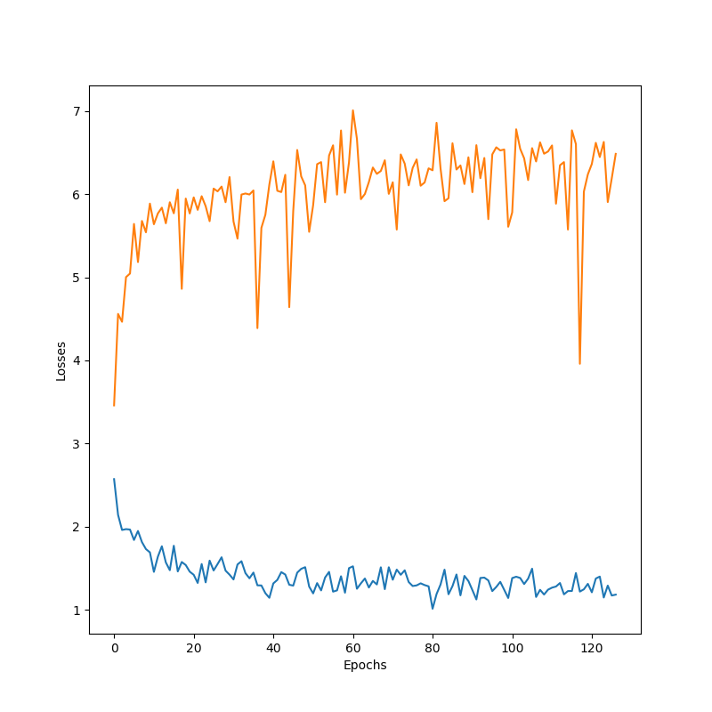
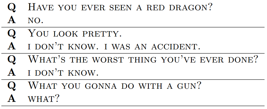
Without Droupout, learning curves produced while training looks like this for most models: 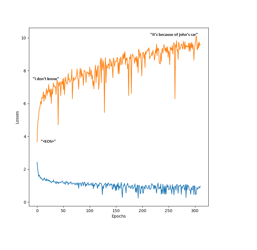curves for the word2word architecture. Each epoch consisted of 250 iterations in which a random mini batch is fed to the network. The labels present on the Figure are standard outputs of the network at different training phases. One common behavior in our experiments was the way networks started of being very boring on the validation set and evolved to being somewhat entertaining on the validation set, despite having a larger loss. This is directly linked to the negative log-likelihood loss function. Therefore, overfitting in the case where we aim at entertaining dialogues with little training data might not be a bad thing. Learning some answers, that are grammatically correct from the training set has at least the advantage of creating less ambiguous answers than “I don’t know” or “Yes”.

Adding attention and dropout

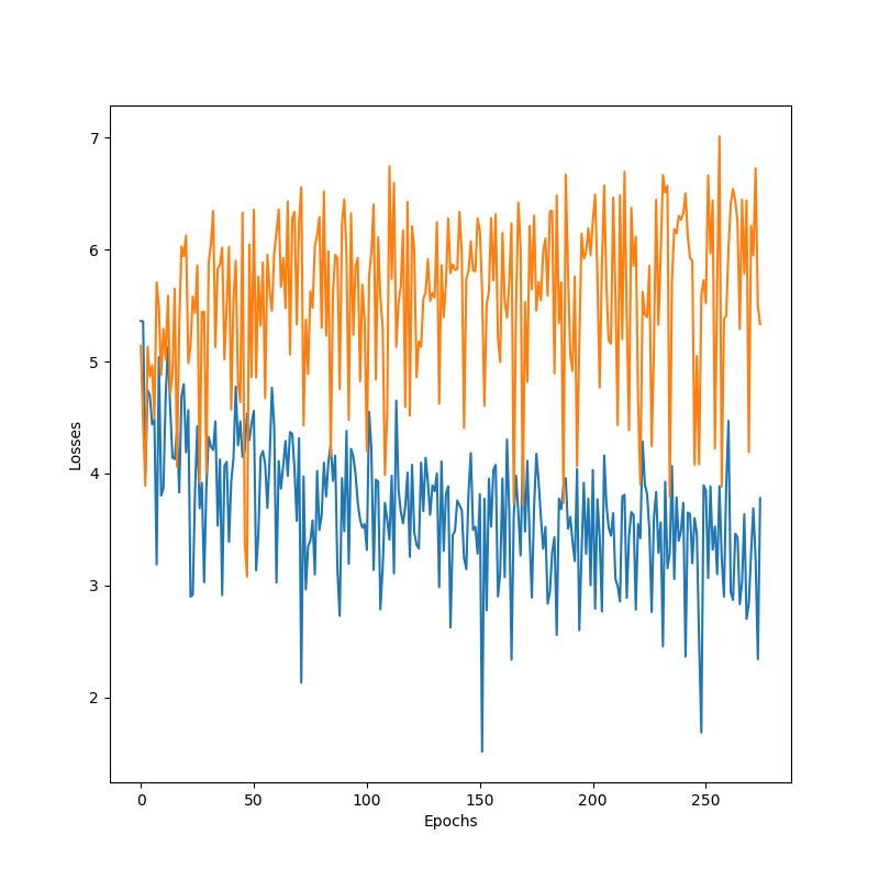
To improve the quality of generated answers, we added the attention mechanism described above, so that it can be easier for the network to use specific words from the question query as conditioning information. Also, we added feed-froward dropout to help generalization of the model. We list here training curves and sample answers for fixed, custom questions for different models, and discuss these results in the Discussion section. When using word-level decoders, we used the sample softmax as described above.

Word2Word

Char2Char

Word2Char

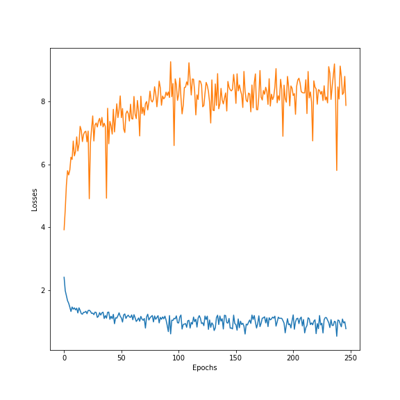
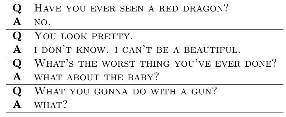
In general, word-level decoders performed worst for answer generations, and char-level decoders learned surprisingly fast to write complete words, as well as punctuation, yielding more realistic sentences. As the curves show, adding attention and dropout seems to help the overall validation performance. However, given the limited data, dropout didn’t allow removing the overfitting occurring almost as soon as training starts.

Capturing style with Messenger

Experiments on the different Messenger datasets were performed mostly out of curiosity and for fun. The main goal here was to assess if a model trained on conversations from one of the authors could capture a bit of his familiar writing style. Indeed, when comparing networks, especially one trained on a French author’s conversation with one trained on a Quebec’s author’s conversations, we could easily assess which network was which. We show some samples below. As explained above, all Messenger bots were trained with char2char architectures.

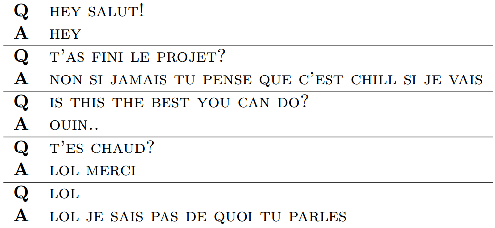
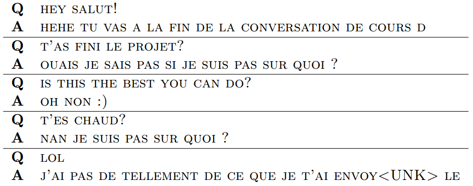
Even with this insufficient number of samples, the third author, whose conversations were not used, could identify which network was trained on whose conversations, showing some level of style captured by the networks. More precisely, key words like “chill” were not present in the French Messenger corpus, and interestingly, word orderings would sometimes not appear in one of the versions, like the word “quoi” following a whole sentence is not common at all in the Quebec corpus. Even though answers were not often of high quality, it shows that the networks learned common language patterns and writing styles.

Conclusion

We implemented a Seq2Seq model for short text generation. The model has been trained of two different datasets, the Cornell Movie Questions and Answers and the author’s Facebook Chat histories. For the Cornell dataset, three variations of the model have been compared : char2char, word2word and word2char. The three models were qualitatively comparable but word2char might provide slightly more sophisticated answers. For the Facebook dataset, only char2char have been implemented due to the unguaranteed grammatical correctness of the data. The model have proven able to capture each author’s style, with especially visible variations between the French and Quebecer styles. Finally, with more time, we would have liked to improve the attention mechanism results and to implement the GAN approach that uses a discriminator to make our generator reply more naturally.

Footnotes

Footnotes 1: For simplicity, let’s define \(\chi(y_k) = w_k^Tf(y_{t-1}, z_t, c_t) + b_k\). Computing the gradient of \(log(p(y_t = y_k|y_{< t}, x))\) gives us \( \nabla(\chi(y_k)) - E_p(\nabla(\chi(y)))\) where the first term is A sparse vector with \(1\) non zero entry at row \(k\), and the second is a complicated sum \(\displaystyle{\sum_{k^{‘}}\frac{\chi(y_{k^{‘}})}{\sum_{k^{‘’}}\chi(y_{k^{‘’}})}\nabla(\chi(y_{k^{‘}}))}\).

Footnotes 2: In a nutshell, importance sampling is a technique to approximate any distribution properties, by sampling from another, usually simpler, distribution.

Footnotes 3: In their paper ¹¹ approximate the expectation with importance sampling by defining a set of distributions \(Q_i\) with their respective subset \(K_i\):

$E_p(\nabla(\chi(y))) = \displaystyle{\sum_{k^{'} \in K^{'}, \|K^{'}\| lt \|K\|}\frac{Q(y_{k^{'}})\chi(y_{k^{'}})}{\sum_{k^{''}}Q(y_{k^{''}})\chi(y_{k^{''}})}\nabla(\chi(y_{k^{'}}))}$ .

Codes

/TODO add

Bibliography

Sébastien Jean and Kyunghyun Cho and Roland Memisevic and Yoshua Bengio