Predicting House Sales using statistical learning technique and deep learning.
Data introduction
Recently, I’ve spent some time learning about R, and I decide to use my rec House Sales In King County. The dataset is available on this page.
The goal of this project will be to predict the price of a house according to characteristics, such as surface area, number of floors, number of rooms
# Import the data
data <- read.csv("kc_house_data.csv")
Let’s have a look at the insight of the data:
head(data)

##           id            date   price bedrooms bathrooms sqft_living
## 1 7129300520 20141013T000000  221900        3      1.00        1180
## 2 6414100192 20141209T000000  538000        3      2.25        2570
## 3 5631500400 20150225T000000  180000        2      1.00         770
## 4 2487200875 20141209T000000  604000        4      3.00        1960
## 5 1954400510 20150218T000000  510000        3      2.00        1680
## 6 7237550310 20140512T000000 1225000        4      4.50        5420
##   sqft_lot floors waterfront view condition grade sqft_above sqft_basement
## 1     5650      1          0    0         3     7       1180             0
## 2     7242      2          0    0         3     7       2170           400
## 3    10000      1          0    0         3     6        770             0
## 4     5000      1          0    0         5     7       1050           910
## 5     8080      1          0    0         3     8       1680             0
## 6   101930      1          0    0         3    11       3890          1530
##   yr_built yr_renovated zipcode     lat     long sqft_living15 sqft_lot15
## 1     1955            0   98178 47.5112 -122.257          1340       5650
## 2     1951         1991   98125 47.7210 -122.319          1690       7639
## 3     1933            0   98028 47.7379 -122.233          2720       8062
## 4     1965            0   98136 47.5208 -122.393          1360       5000
## 5     1987            0   98074 47.6168 -122.045          1800       7503
## 6     2001            0   98053 47.6561 -122.005          4760     101930
# Number of examples
nrow(data)
## [1] 21613
# Number of features
ncol(data)
## [1] 21
This database is made up of a substantial number of examples, which makes it possible to train several models of prediction, and to separate our data into a training set and a validation set.
Data preprocessing
Selecting attributes
Some data are not compelling at all to predict the price, then removing them is legitimate; I am talking about the id, the date, the zipcode, lattitude, and longitude. It seemed to me that it leads to potential confusion for training our models.
data = data[,-c(1:2, 17:19)]
Removing outlier
Removing outliers improve the quality and generalization of trained models. For example, it reduces the variance. As there are many examples, removing some of them is possible. Hence, we’ll remove all outlier of surfaces and price attributes. Also, the explanatory variable * prices * will be deleted. In fact, in Our database is indeed found costly houses, which are usually outlier with a price very different from the rest. Hence they won’t fit any linear model. On the opposite, meager price, is hard to predict for any model. If the model is sufficiently flexible, it may be possible to predict the price of these examples, but this is not what we want. We want a good generalization, not an overfitted model.
remove_outliers <- function(x, na.rm = TRUE, ...) {
  qnt <- quantile(x, probs=c(.25, .75), na.rm = na.rm, ...)
  H <- 4 * IQR(x, na.rm = na.rm)
  y =
    y = c(which(x < (qnt[1] - H)),which(x > (qnt[2] + H)))
  y
}
num = 0
for(name  in names(data)){
  if(grepl("sqft", name) || name == "price"){
    outliers = remove_outliers(data[,name])
    num = num + length(outliers)
    data = data[-outliers,]
  }
}
# Number of data removed
print(num)
## [1] 2030

# Number of daa still available
print(nrow(data))
## [1] 19583
Removing abortive data will, of course, reduce the RSS, MSE calculated from our data. But this will undoubtedly help models converge towards a solution that will generalize better.
Decoralleted features
In order to avoid having too correlated features, it is necessary to remove one of the two variables of the attributes pairs that have an higher correlation than 0.75. Sub-model selection methods had a drop in performance when the explanatory variables are too correlated.
tmp = cor(data)
tmp[lower.tri(tmp)] = 0
diag(tmp) =  0
data1 = data[, !apply(tmp, 2, function(x) any(x > 0.75))]
setdiff(names(data), names(data1))

## [1] "sqft_above"    "sqft_living15" "sqft_lot15"
Three variables were removed from the model. These are sqft_above, sqftliving15, sqft_lot15. They are indeed very correlated with the variable sqft_living.
Transforming numerical data
All data is numeric. Variables such as bathrooms, bedrooms, floors will be left as a numeric variable, because the difference between these values is interpreted relatively well, and it won’t harm any model. However, it’s not the case of variables like condition, view and grade. Condition has three maximum factors, while grade has at least five. So it is better to convert them as dummy variables. A function is created for it.
as.dummy_variable = function (data){
  data$floor = factor(data$floor)
  data$view = factor(data$view)
  data$condition = factor(data$condition)
  data$grade = factor(data$grade)
  return(data)
}
Splitting between training and testing time
The data will be separated into two groups, the training of our models. For this, the * sample * method will be used:
smp_size = floor(0.7 * nrow(data))
train_ind = sample(seq_len(nrow(data)), size = smp_size)
train = data[train_ind,]
test = data[-train_ind,]
Some statistics
The function summary will be used and get some statistics on our explanatory variables (mean, minimal, maximal, variance, median)
summary(data)

##      price            bedrooms        bathrooms      sqft_living
##  Min.   :  78000   Min.   : 0.000   Min.   :0.000   Min.   : 290
##  1st Qu.: 315000   1st Qu.: 3.000   1st Qu.:1.500   1st Qu.:1400
##  Median : 439000   Median : 3.000   Median :2.250   Median :1850
##  Mean   : 506314   Mean   : 3.348   Mean   :2.071   Mean   :1988
##  3rd Qu.: 620000   3rd Qu.: 4.000   3rd Qu.:2.500   3rd Qu.:2440
##  Max.   :1928000   Max.   :33.000   Max.   :7.500   Max.   :6630
##     sqft_lot         floors        waterfront            view
##  Min.   :  520   Min.   :1.000   Min.   :0.000000   Min.   :0.0000
##  1st Qu.: 4976   1st Qu.:1.000   1st Qu.:0.000000   1st Qu.:0.0000
##  Median : 7245   Median :1.000   Median :0.000000   Median :0.0000
##  Mean   : 7824   Mean   :1.487   Mean   :0.004136   Mean   :0.2046
##  3rd Qu.: 9604   3rd Qu.:2.000   3rd Qu.:0.000000   3rd Qu.:0.0000
##  Max.   :32481   Max.   :3.500   Max.   :1.000000   Max.   :4.0000
##    condition         grade        sqft_basement       yr_built
##  Min.   :1.000   Min.   : 1.000   Min.   :   0.0   Min.   :1900
##  1st Qu.:3.000   1st Qu.: 7.000   1st Qu.:   0.0   1st Qu.:1950
##  Median :3.000   Median : 7.000   Median :   0.0   Median :1972
##  Mean   :3.411   Mean   : 7.565   Mean   : 282.7   Mean   :1970
##  3rd Qu.:4.000   3rd Qu.: 8.000   3rd Qu.: 550.0   3rd Qu.:1997
##  Max.   :5.000   Max.   :12.000   Max.   :2610.0   Max.   :2015
##   yr_renovated
##  Min.   :   0.00
##  1st Qu.:   0.00
##  Median :   0.00
##  Mean   :  79.92
##  3rd Qu.:   0.00
##  Max.   :2015.00
Simple regression with a single explanatory variable
The explanatory value used will be the most numerical correlated with the price variable:
cor_matrix = cor(data)
cor_matrix[,"price"]

##         price      bedrooms     bathrooms   sqft_living      sqft_lot
##    1.00000000    0.30598400    0.48186574    0.66031611    0.11239660
##        floors    waterfront          view     condition         grade
##    0.26696595    0.14587787    0.36062051    0.05249493    0.66324669
## sqft_basement      yr_built  yr_renovated
##    0.30394940    0.02994293    0.13446924
The most correlated numerical explanatory variable is sqft-living.
Price as a function of the living surface
lm.fit =lm(price ~ sqft_living, data=train)
summary(lm.fit)

##
## Call:
## lm(formula = price ~ sqft_living, data = train)
##
## Residuals:
##     Min      1Q  Median      3Q     Max
## -752305 -138675  -21914  101686 1243428
##
## Coefficients:
##              Estimate Std. Error t value Pr(>|t|)
## (Intercept) 53371.070   4714.600   11.32   <2e-16 ***
## sqft_living   227.143      2.197  103.37   <2e-16 ***
## ---
## Signif. codes:  0 '***' 0.001 '**' 0.01 '*' 0.05 '.' 0.1 ' ' 1
##
## Residual standard error: 206900 on 13706 degrees of freedom
## Multiple R-squared:  0.4381, Adjusted R-squared:  0.438
## F-statistic: 1.069e+04 on 1 and 13706 DF,  p-value: < 2.2e-16

lm.pred = predict(lm.fit, test)
lm.rmse = sqrt(mean((lm.pred - test$price) ^2) )
# Racine carée du MSE du modéle
lm.rmse

## [1] 209455.5
According to the adjusted \(R^2\), the variance in the house price is hardly explained by the data sqft-living. However, the RMSE is high, indicating that the simple linear model is probably incomplete, or too simple. Here is the scatter plot.
pairs(data[, c(1,4)])
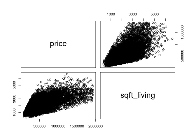
Looking at the curve, it appears that price variability increases with the common area. It is possible to transform linearly the variable sqftliving to see if this improves the quality of the regression.
lm.fit =lm(price ~  I(sqft_living ^ (2)), data=train)
summary(lm.fit)

##
## Call:
## lm(formula = price ~ I(sqft_living^(2)), data = train)
##
## Residuals:
##      Min       1Q   Median       3Q      Max
## -1100069  -137821   -26246    98835  1280545
##
## Coefficients:
##                     Estimate Std. Error t value Pr(>|t|)
## (Intercept)        2.906e+05  2.708e+03   107.3   <2e-16 ***
## I(sqft_living^(2)) 4.663e-02  4.470e-04   104.3   <2e-16 ***
## ---
## Signif. codes:  0 '***' 0.001 '**' 0.01 '*' 0.05 '.' 0.1 ' ' 1
##
## Residual standard error: 206100 on 13706 degrees of freedom
## Multiple R-squared:  0.4425, Adjusted R-squared:  0.4424
## F-statistic: 1.088e+04 on 1 and 13706 DF,  p-value: < 2.2e-16

lm.pred = predict(lm.fit, test)
sqrt(mean((lm.pred - test$price) ^2) )

## [1] 208662.5
After testing several nonlinear modifications to sqft_living (sqrt, log, \(^2\), \(^3\)), none seems to improve the regression.
LASSO regression
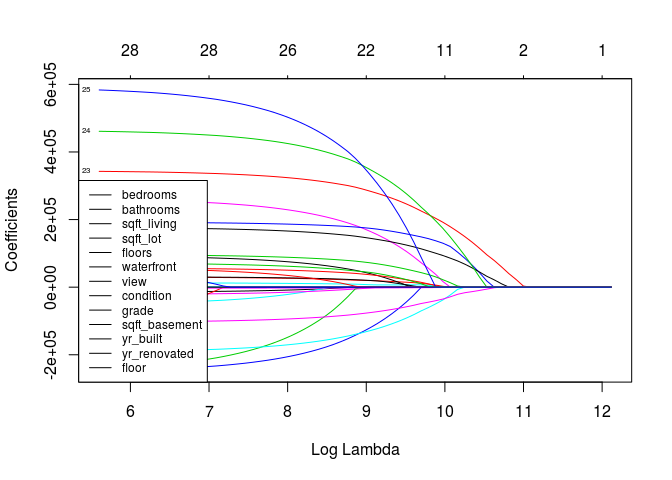
The advantage of the LASSO regression is that it allows selecting among the explanatory variables those that best explain the dependent variable. If the LASSO coefficient β of any explanatory variable tends to zero, then the variable can not influence the prediction of the dependent variable. Depending on the results of the algorithm, some explanatory variables will be removed from the model.
# Transformer les données non numériques en dummy variable
data = as.dummy_variable(data)
train = data[train_ind,]
test = data[-train_ind,]

# LASSO REGRESSION MODEL
x = model.matrix(price ~., data=train)
y = train[,1]
fit.lasso = glmnet(x, y, alpha = 1)
plot(fit.lasso, xvar="lambda", label=T)
legend("bottomleft", names(train[-1]), lty=1, cex=.75)
# Optima value of LAMBDA
cv.lasso = cv.glmnet(x,y, alpha=1)
plot(cv.lasso)
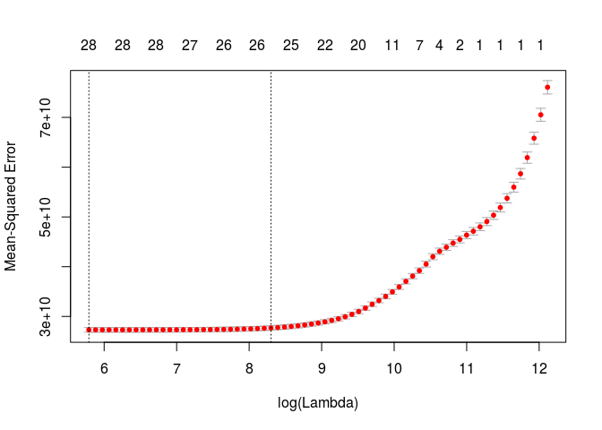
lambda.min = cv.lasso$lambda.min
print(lambda.min)

## [1] 326.739

fit.lasso = glmnet(x, y,alpha = 1, lambda = lambda.min)
fit.pred = predict(fit.lasso, model.matrix(price~.,data=test))
print(paste("RMSE : ", sqrt(mean((fit.pred - test$price) ^ 2))))

## [1] "RMSE :  164778.582907721"

# Coefficient des variables explicatives
coef.lasso = coef(cv.lasso)
coef.lasso

## 34 x 1 sparse Matrix of class "dgCMatrix"
##                           1
## (Intercept)    5.357123e+06
## (Intercept)    .
## bedrooms      -6.316303e+03
## bathrooms      2.477882e+04
## sqft_living    1.223387e+02
## sqft_lot      -3.432196e+00
## floors         1.047572e+04
## waterfront     2.170895e+05
## view1          6.868382e+04
## view2          4.775761e+04
## view3          8.550401e+04
## view4          1.843535e+05
## condition2    -1.091966e+04
## condition3    -1.250071e+04
## condition4     .
## condition5     2.613684e+04
## grade3         .
## grade4        -1.125385e+05
## grade5        -1.898672e+05
## grade6        -1.627385e+05
## grade7        -9.070637e+04
## grade8         .
## grade9         1.621404e+05
## grade10        3.167587e+05
## grade11        4.110048e+05
## grade12        4.716455e+05
## sqft_basement  7.570816e+00
## yr_built      -2.588052e+03
## yr_renovated   1.174276e+01
## floor1.5       .
## floor2         .
## floor2.5       2.646550e+04
## floor3         5.832920e+04
## floor3.5       .
For an optimal value of \(\lambda = 326.739\) given by cross_validation un lambda optimal obtenue par la méthode de cross validation, coefficients of sqft_lot, sqft_basement, yr.renovated are closed to zeros, hence we can remove thoses variables from future regression models.
data = data[, -c(5, 11, 13)]
train = data[train_ind,]
test = data[-train_ind,]
Best subset models
# FORWARD STEPWISE SELECTION
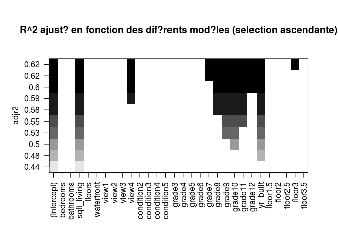
regfw.subset = regsubsets(price ~ ., train, nbest = 1, nvmax = ncol(data)-1, method= "forward")

regfwd.summary = summary(regfw.subset)
plot(regfw.subset, scale = "adjr2")
# BACKWARD STEPWISE SELECTION
regfw.subset = regsubsets(price ~ ., train, nbest = 1, nvmax = ncol(data)-1, method= "backward")

regfwd.summary = summary(regfw.subset)
plot(regfw.subset, scale = "adjr2", main = "R^2 ajusté en fonction des diférents modéles (selection descendante)")
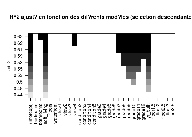
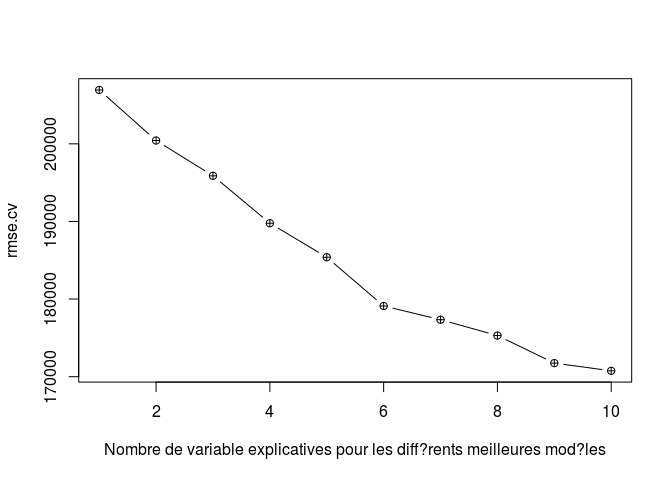
Selection of the best model using cross validation.
# CROSS VALIDATION
folds = sample(rep(1:10, length = nrow(train)))
cv.errors = matrix(NA, 10, ncol(data) - 1)

prediction.regsubsets = function(object, newdata, id, ...){
  form = as.formula(object$call[[2]]) #extract object model formula for y ~ x
  mat = model.matrix(form, newdata) #set prediction matrix
  coefi = coef(object, id = id) #obtain matrix of coefficients
  mat[, names(coefi)] %*% coefi #calculate predictions matrix
}

for(k in 1:10){
  best.fit = regsubsets(price ~ .  , data = train[folds != k, ], nvmax = ncol(data)-1,
                        method = "forward")
  for(i in 1:(ncol(data)-1)){
    pred = prediction.regsubsets(best.fit, train[folds == k, ], id = i)

    cv.errors[k, i] = mean((train$price[folds == k] - pred) ^ 2)
  }
}

# Reordering variables and trying again:
rmse.cv = sqrt(apply(cv.errors, 2, mean))
plot(rmse.cv, pch = ncol(data)-1, type = "b",xlab = "Nombre de variable explicatives pour les différents meilleures modéles")
# Best model over the training set
which.min(rmse.cv)

## [1] 10
The best-validated model is, therefore, the model 10, it will be used on our test data.
x.test = model.matrix(price ~., data = test)

# Calculer le MSE pour tous les modéles (et voir si le modéle choisi minimise le MSE des données de test)
coefi = coef(regfw.subset, id = 10)
pred = x.test[ , names(coefi)] %*% coefi
paste("Modele 10, RMSE = ",sqrt(mean((test$price - pred) ^ 2)))

## [1] "Modele 10, RMSE =  171457.71092754"
Compared to the simple regression model, an explanatory variable, the RMSE test has decreased by 30,000. This is partly explained by the fact that the last model is more flexible.
PCA
The approach of the main components is another statisticals technique to find the variables Xi of the model which explains the maximum variance of the dependent variable.
pcr.fit = pcr(price ~., data=data, scale=T, validation="CV", ncomp=27)
summary(pcr.fit)

## Data:    X dimension: 19583 29
##  Y dimension: 19583 1
## Fit method: svdpc
## Number of components considered: 27
##
## VALIDATION: RMSEP
## Cross-validated using 10 random segments.
##        (Intercept)  1 comps  2 comps  3 comps  4 comps  5 comps  6 comps
## CV          276527   243636   205658   201720   201623   197521   196540
## adjCV       276527   243635   205645   201699   201606   197500   196523
##        7 comps  8 comps  9 comps  10 comps  11 comps  12 comps  13 comps
## CV      195857   192119   191811    191778    191749    191070    190893
## adjCV   195858   191866   191772    191784    191790    191020    190961
##        14 comps  15 comps  16 comps  17 comps  18 comps  19 comps
## CV       190672    190386    190048    189708    189251    188639
## adjCV    190682    190315    189983    189860    189237    188629
##        20 comps  21 comps  22 comps  23 comps  24 comps  25 comps
## CV       188502    188433    178661    178591    167097    166197
## adjCV    188483    188414    178635    178578    167075    166177
##        26 comps  27 comps
## CV       166213    166228
## adjCV    166193    166206
##
## TRAINING: % variance explained
##        1 comps  2 comps  3 comps  4 comps  5 comps  6 comps  7 comps
## X        15.22    22.23    27.71    32.84    37.47    41.81    45.81
## price    22.39    44.72    46.83    46.91    49.05    49.56    49.91
##        8 comps  9 comps  10 comps  11 comps  12 comps  13 comps  14 comps
## X        49.67    53.47     57.11     60.69     64.23     67.73     71.20
## price    51.97    51.97     51.97     51.99     52.44     52.44     52.56
##        15 comps  16 comps  17 comps  18 comps  19 comps  20 comps
## X         74.64     78.05     81.45     84.83     88.03     91.07
## price     52.77     52.95     52.96     53.31     53.64     53.73
##        21 comps  22 comps  23 comps  24 comps  25 comps  26 comps
## X         93.73     95.61     97.13     98.40     99.41     99.99
## price     53.77     58.42     58.45     63.64     64.03     64.04
##        27 comps
## X        100.00
## price     64.04

validationplot(pcr.fit, val.type = "RMSEP")
 The optimal value M of the number of explanatory variables is 27. However, we note that from 24 variables, the RMSE, as well as variance of the model are close to the optimal value. As a result, M = 24 will be used to measure our MSE on the test set.
pcr.fit = pcr(price ~ ., data=train, scale=T, validation="CV", ncomp= 24)
pcr.pred = predict(pcr.fit, test, ncomp = 24)
sqrt(mean((pcr.pred - test$price) ^2))

## [1] 167071.6
Regression tree
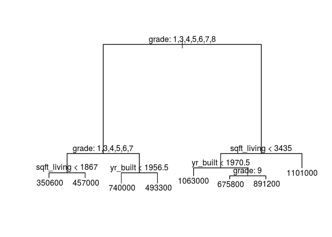
The last technique used will be regression trees. Let’s start with a single regression tree.
tree.fit = tree(price~., data=train)
summary(tree.fit)

##
## Regression tree:
## tree(formula = price ~ ., data = train)
## Variables actually used in tree construction:
## [1] "grade"       "sqft_living" "yr_built"
## Number of terminal nodes:  8
## Residual mean deviance:  3.515e+10 = 4.815e+14 / 13700
## Distribution of residuals:
##    Min. 1st Qu.  Median    Mean 3rd Qu.    Max.
## -758400 -122300  -28350       0   93680 1358000

plot(tree.fit)
text(tree.fit, pretty=0)
tree.pred = predict(tree.fit, test)
sqrt(mean((test$price - tree.pred)^2))

## [1] 191385.4
With the method of cross validation, it is possible to determine an optimal tree size. R provides a function for this cv.tree.
plot(tree.cvsize, tree, cvdev, type="b")

tree.min = which.min(tree.cv$size)
tree.min
The optimal depth obtained above corresponds to the initial depth of our tree. The RMSE is high, compared to the scores of the other methods; doubly because using a single tree to predict the price is highly variant.
Random Forest improves a lot the uses of regression trees, recovering the result of several regression trees, constructed differently, independently, using bootstrapped data. It has the effect of reducing a lot the variance of the initial method. Each split in each tree is computed from some attributes m < number of total preachers. Here are the results for m = 5.
rf.fit = randomForest(price~., data=train, mtry=5, ntree=50, importance=TRUE)
rf.pred = predict(rf.fit, test)
sqrt(mean((test$price - rf.pred)^2))

## [1] 163452.1
The RMSE is much better than for a single tree, which seems logical. This method gets the best score on the RMSE test.
Neural networks
Finally, I wanted to try neural network and see if it will beat the current best RMSE test. I didn’t. Even worse, it fails entirely. I was not able to conclude the reason for this failure because neural networks are always tricky to debug, even though they are sometimes very powerful.
Moreover, in our cases, attributes are already engineered. Hence we can use simpler model other than neural network, which is very powerful to do the feature processing at every layer, for us.
At the end of 100 eras (passage on the data) is ~180000.
Conclusion
Resume
After cleaning our initial data set, by removing unuseful attributes, decorrelating those remaining, and removing Outliers, we were able to train several models. Each model predicted the price of the house according to a dozen of attributes maximum. The simple linear regression of the price as a function of the surface allowed us to establish a baseline minimum error score of RMSE test: 208662.5). Then, we used more complex models.
- Lasso regression (RMSE test: 164778.5)
- The approach of the best subsets (RMSE test: 171457.7),
- The principal components approach (RMSE test: 167071.6),
- 1 tree of regression (RMSE test: 191385.4)
- Random forest (RMSE test: 162527.1).
Analyse
This percentage of error is high, but the exact price of a house at the scale of a large geographic area is quite complicated, and some features were not taken into account (such as leasing). Moreover, the models used assumed a linear relationship between the predicates, and the output variable, which is not necessarily the case, given the best performance obtained by the random forest technique.
Kaggle comparison on RMSE test
By comparing, results obtained with those from the best ranked script, It appears that I get better prediction than their model. The difference might comes from better preprocessing.